
Note
Go to the end to download the full example code.
Orthographic comparison#
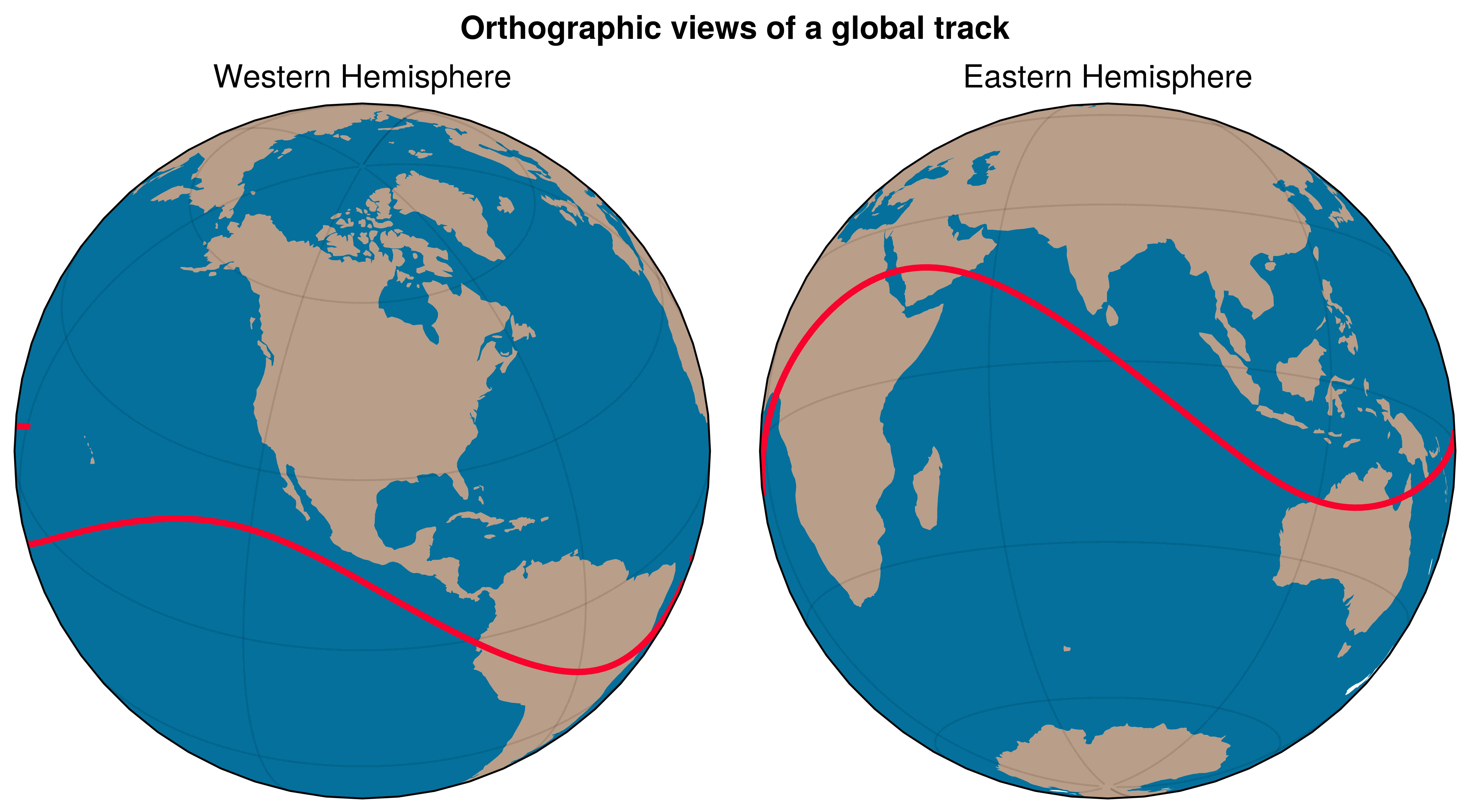
Two orthographic views of the same signal to emphasize projection control.
Why UltraPlot here?#
UltraPlot handles multiple projections in one figure with a consistent API and shared formatting calls. This makes side-by-side map comparisons simple.
Key functions: ultraplot.figure.Figure.subplot(), ultraplot.axes.GeoAxes.format().
See also#
import cartopy.crs as ccrs
import numpy as np

import ultraplot as uplt

lon = np.linspace(-180, 180, 220)
lat = 20 * np.sin(np.deg2rad(lon * 2.2))

fig = uplt.figure(refwidth=3, share=0)
ax1 = fig.subplot(121, proj="ortho", proj_kw={"lon0": -100, "lat0": 35})
ax2 = fig.subplot(122, proj="ortho", proj_kw={"lon0": 80, "lat0": -15})

for ax, title in zip([ax1, ax2], ["Western Hemisphere", "Eastern Hemisphere"]):
    ax.plot(lon, lat, transform=ccrs.PlateCarree(), lw=2, color="cherry red")
    ax.scatter(lon[::40], lat[::40], transform=ccrs.PlateCarree(), s=30)
    ax.format(
        lonlines=60,
        latlines=30,
        title=title,
        land=True,
        ocean=True,
        oceancolor="ocean blue",
        landcolor="mushroom",
    )

fig.format(suptitle="Orthographic views of a global track")

fig.show()
Total running time of the script: (0 minutes 2.845 seconds)